Fourier Series representation of a periodic waveform is handy. Do you really believe it?
1. Setup
1.1. Materials
-
LTspice installed
-
Or CircuitLab
-
Ulaby book, Chapter 13. pdf pages 689-691
1.2. Objectives
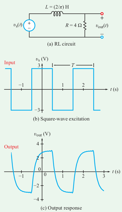
Reproduce the example in Ulaby section 13-1 using a circuit simulator.
-
Use a circuit simulator to simulate the circuit of Ulaby Figure 13-1(a)
-
with the input of the waveforms in Ulaby Figure 13-1(b)
-
and displaying the output waveform of Figure 13-1(c).
-
Then reproducing the output waveform of Figure 13-1(c) using its Fourier Series representation.
Concepts:
-
Fourier series of a square wave of certain amplitude and frequency.
-
Phasor analysis of an LR circuit
1.3. Setup LTspice
The default keyboard shortcuts for LTspice need improvement. This two-minute video shows how to make them better:
The files referenced may be found at:
1.4. Fourier theorem
A periodic waveform that satisfies the Dirichlet conditions_ with a period of T may be represented as:
Remember: \(\omega_0 = \dfrac{2\pi}{T}\)
2. General procedure
Read book section 13-1 first! Then it will become a reference for everything else today.
Draw the circuit of Figure 13-1(a) in LTspice.
Create a .tran(sient) simulation for 5 seconds and plot the voltage source and vout.

Right click on the voltage source, then the Advanced button to get to the square wave settings.
Figure out what settings you need to make your waveform match Figure 13-1(b). Don’t continue until these match!
Create a series stack of sine sources of appropriate magnitudes, frequencies, and phases to obtain the FS representation of the input square wave. Remember that LTspice uses sin() while the math version uses cos().
Apply this composite voltage source to a second identical LR circuit to demonstrate the output is also similar to the original.
Create a second series stack of sources to directly approximate the output waveform. Book secion 13-1 includes the general form for finding the magnitudes and phases already for this particular input and circuit.
-
How many terms or sinusoids do you need for a "good" approximation?
A rule-of-thumb for seeing a reasonable square wave on an oscilloscope is for the 'scope to have a bandwidth for the 5th harmonic (5f0).
-
Given this rule of thumb, what is the maximum frequency of an input square wave your Analog Discovery 2 can display with good fidelity?
3. Submission
Submit your LTspice .asc schematic which simulates:
-
The original square wave and corresponding LR circuit output.
-
A FS approximation to a square waveform.
-
This approximation sent through an LR circuit showing the approximated output waveform.
-
A FS approximation of the output directly obtained from circuit analysis using the input series and phasors. This should match #3 exactly.