1. Objective
In this lab, we will investigate the effects of temperature on electronic devices: resistors that change value with temperature and inferring the amount of thermally-generated free charge carriers by measuring the reverse-bias current through a diode.
NOTE: Do not skim-read the procedure. The wording is precise and specific, skipping steps or missing things will guarantee you will not finish your measurements within the scheduled lab time. Many problems will be avoided if you do not try to rush through the procedure.
READ THE PROCEDURE CAREFULLY slow down…!
2. Theory
| Skip this section for now and start with the Procedure section. Go back and read this while waiting for your measurements to stabilize. |
2.1. Silicon pn junction diode
The silicon pn junction diode has an ideal current-voltage relationship of:
The term \(k_B T /q\) is known as the thermal voltage \(V_T\) and is approximately \(26 \mathrm{mV}\) at room temperature, \(n\) is called the ideality factor and is 1 for an ideal diode but larger (1—2 range) for a real diode. \(I_S\) is called the saturation current. For reverse-bias (negative) voltages larger than a few hundred \(\mathrm{mV}\), the diode current can be approximated as \(\approx -I_S\) (can you see why this is?).
In addition to the \(1/T\) term directly in the equation’s exponential, the saturation current \(I_S\) is a strong function of temperature. It can be calculated from geometrical and material parameters as:
where \(A\) is the device’s cross-sectional area, \(L_n\) and \(L_p\) are electron and hole “diffusion lengths,” respectively, \(D_{n,p}\) are the electron and hole diffusion constants, and \(N_{A,D}\) are the doping concentrations for the p and n sides of the junction. These parameters can be treated as constants in this discussion.
The Einstein Relation can be proven to relate the ratio of the diffusion constant to mobility in a material as:
Solving for the diffusion constant, \(D_{n,p} = \mu_{n,p} \dfrac{k_B T}{q}\), re-write the saturation current and factor out temperature:
Ignore the fact that mobility still changes with temperature due to several other effects — it reaches a maximum at an intermediate temperature.
The intrinsic carrier density also varies with temperature:
We are only interested in the temperature dependence of \(I_S\) for a specific device, so collapse all the temperature-independent terms into a single constant:
2.2. Thermistors
The resistivity of all materials varies with temperature, and different types of resistor materials have varying sensitivities to temperature. This change in resistance over temperature for “normal” resistors is specified as its temperature coefficient of resistance (TCR) and has units of percent or PPM (parts-per-million) per degree. Usually, \(T_{ref}\) is room temperature.
See the following link for more information: Temperature Coefficient of Copper
Thermistors are devices which are designed to change their resistance with temperature. Their obvious application is to measure temperature. Other interesting applications include measurement of air speed and density in aircraft as the airstream cools the device. Their resistance is dependent on temperature as approximately:
where \(B\) is a constant for the specific device, \(T_R\) is the rated temperature, and \(R_R\) is the resistance at the rated temperature. The thermistors used in this lab are specified as \(1\mathrm{k\Omega}\) at \(25^\circ C\) (\(R_R=1k\) and \(T_R=25^\circ C\)) with constant \(B = 3930 K\). Be mindful of the temperature units in your calculations (\(0^\circ C = 273.15 K\)).
See the file NTC-general-technical-information.pdf for more background information and NTC_Leaded_disks_M891.pdf for the specific values.
A more accurate determination of resistance or temperature is obtained from using actual values and temperatures provided in tables in the device’s datasheet and interpolating between the values.
Page 2 of the NTC-standardizedrt.pdf file describes the calculations and gives an example.
We are using the \(1 \mathrm{k\Omega}\) rated thermistor, whose data table is number “1009” in the datasheet, file NTC_Leaded_disks_M891.pdf.
These files may be found in the course’s Google Drive docs folder.
3. Procedure
The general format of these instructions is: the first 1-2 sentences are your task to do and the rest is a short description of why.
Goal: Setup your oscilloscope to precisely measure very small DC values in the presence of noise and interference.
-
Adjust both outputs of the benchtop power supply to \(0\,\mathrm{V}\) before attaching your circuit..
-
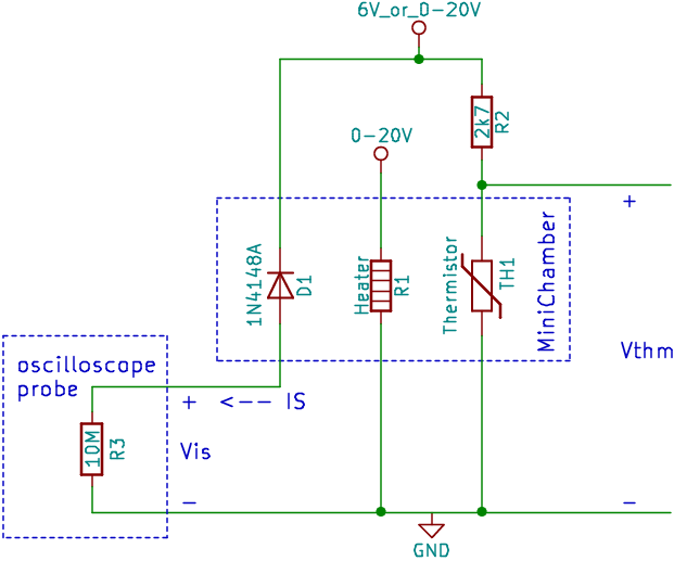
Connect the \(+6\,\mathrm{V}\) power supply terminal to the node labeled
6V_or_0-20Von the schematic. -
Connect the \(+20\,\mathrm{V}\) power supply terminal to the node labeled
0-20Von the schematic. -
Connect the
COMterminal of the power supply to the node labeledGNDon the schematic.
-
Connect oscilloscope channel 1’s “+” terminal (the tip) to the anode side of the diode and the black ground clip lead to the node labeled
GND.-
This makes it appear that channel 1 is connected across nothing, which is not necessarily intuitive. The currents we will be measuring will initially be a few \(\mathrm{nA}\), a million times below the range of cheap ammeters (the nice multimeters can measure this). With this connection scheme, the diode is in series with the probe and therefore the saturation current \(I_S\) goes through the \(10 \,\mathrm{M\Omega}\) input resistance of the oscilloscope+probe combination. Using a resistor to measure current in this way is called a current shunt. The voltage measured across this resistance by the scope is proportional to the current through it via Ohms law. This current \(I_S\) is labeled on the schematic.
-
-
Connect oscilloscope channel 2’s “+” terminal to the node between the MiniChamber’s thermistor and the \(2.7 \,\mathrm{k\Omega}\) resistor. Connect the ground lead to the
GNDnode. -
Turn on the power supply. The outputs should already have been both set to zero.
-
Raise the \(+6\,\mathrm{V}\) power supply output to about \(+6\,\mathrm{V}\) and record the actual value shown on the power supply’s meter. It is not critical to be at exactly \(6.00\), but it is important to use the true measured value for your data collection and calculations.
-
Touch the “Default Setup” key on the scope, then select the “Factory Default” option in the soft menu (confirm that you want to reset to factory settings). This completely resets your scope’s settings. Default Setup alone still leaves some settings unchanged.
-
Touch the “Acquire" key on the scope and change the Acquire Mode to "High Res”. The manual says the scope displays the average of the many samples taken by the front-end for each displayed pixel in this mode. “Normal” mode merely displays the first sample value in the interval.
-
Change the trigger system to trigger on the edge of the “Line” source. The signal you see is the superposition of the DC value to be measured, random noise, and induced voltage from the \(60 \,\mathrm{Hz}\) electric and magnetic fields in the room from the building power. The signals we are interested in are DC only, but the probe will pick up a large amount of powerline interference as you can see on the screen. This keeps the interference on the display stable so we can then average-out the display and make more precise measurements because all of the interference has a zero mean.
-
Change the vertical scale and vertical position of both channels (\(V_{thm}\) and \(V_{I_S}\)) to show both the entire signal waveform and the channel’s \(0 \,\mathrm{V}\) reference level on the screen. The goal is to maximize the amount of (vertical) screen area that the signal occupies while still showing its magnitude above zero. This gives you the most accurate measurements.
-
Change the horizontal scale to show 5-8 periods of the \(60 \,\mathrm{Hz}\) interference waveform.
-
Using the measurement functions, display the full-screen averages of both channel voltages. Average and DC are synonomous—computing the average is the same as finding the DC value of a signal. Do not be deceived by the "DC" text in some of the other measure menu items!
-
Observe these measurements and record the values when they stop slowly changing up or down.
Goal of this section: Measure the DC values of \(V_{thm}\) and \(V_{I_S}\) at different temperatures. \(V_{thm}\) allows you to compute the current temperature and \(V_{I_S}\) is directly related to the diode’s reverse-bias current.
The 6V_or_0-20V connection applies a reverse-bias voltage across the diode to create this current.
We switch the power supply connection to that node since we don’t have an extra \(20\,\mathrm{V}\) power supply output and because both GND leads of the oscilloscope channels must be connected to the same node (a limitation of the bench-top 'scopes).
-
Increase the \(0-20 \,\mathrm{V}\) power supply output in \(2.0 \,\mathrm{V}\) increments until it reaches \(6.0 \,\mathrm{V}\) and then use \(1.0 \,\mathrm{V}\) increments. (0, 2, 4, 6, 7, 8, 9, …)
-
At each increment, wait for the temperature to reach equilibrium. Calculate your wait time for each measurement that allows you to finish all your measurements by 10 minutes before the lab session ends.
-
These changes will be slow and small at first. \(V_{I_S}\) will be around \(40 \,\mathrm{mV}\) at the beginning.
-
At the end of each increment’s time interval, record 5 data values:
-
The \(20 \mathrm{V}\) supply voltage
-
The \(20 \mathrm{V}\) supply current
-
The voltage at the node labeled
6V_or_0-20V. -
\(V_{I_S}\) (oscilloscope channel 1)
-
\(V_{thm}\) (oscilloscope channel 2)
-
-
When the \(20 \,\mathrm{V}\) supply increment reaches \(6 \,\mathrm{V}\): Move the power supply connection to node labeled
6V_or_0-20Vfrom the \(6\,\mathrm{V}\) output to the \(20 \,\mathrm{V}\) output. The diode, heater, and \(2.7 \,\mathrm{k\Omega}\) resistor will therefore all be connected to the \(20 \,\mathrm{V}\) output and the \(6 \mathrm{V}\) power supply will then be disconnected. -
Stop the experiment when either the thermistor reaches the calculated resistance for \(100 \,\mathrm{^\circ C}\) or the MiniChamber appears to be becoming damaged (smoke, noise, etc.).
-
-
While waiting for each measurement to stabilize: setup your calculations and plots, viewing each new data point as you enter them. It is useful to pre-define the “plot range” to be the full number of rows you expect to have, this way you do not need to update that range for each new data point.
-
Calculate what the thermistor’s resistance will be at \(100 \mathrm{^\circ C}\) using Equation 9. This is the maximum temperature the MiniChamber should reach with the corresponding thermistor resistance.
-
Done! Return your MiniChamber, cleanup your lab station, and make sure the proper number and type of cables are returned to the storage box.
4. Analysis
Use Excel or Google Sheets to perform these calculations.
-
Using circuit analysis and the thermistor datasheet, determine the thermistor resistance and therefore temperature for each of your \(V_{thm}\) measurements. You can calculate the expected value of \(V_{thm}\) at room temperature, when the thermistor resistance is around \(1 \,\mathrm{k\Omega}\).
-
Calculate the heat power dissipated by the heater resistor and supplied to the system at each measurement point.
-
Using circuit analysis, calculate the diode saturation current \(I_S\) as measured by the oscilloscope probe \(V_{Is}\). (Technically we are measuring the diode’s leakage current instead, which includes a few more temperature-related effects.)
-
From the heater resistor’s applied voltage and resulting measured current, calculate the heater’s effective resistance. It also changes with temperature :(
At this point, your spreadsheet will have 5 columns of raw data, and 5 columns of calculated values from this data. Keep the columns in separate groups to visually differentiate between raw data measurements and derived numbers; this is good lab practice.
From the numbers, generate the following plots: (remember: “\(y\) vs. \(x\)”)
-
\(I_S\) vs. temperature
-
On this figure, also plot the theoretical value of \(I_S\) versus temperature. Choose the constants \(C\) and \(n\) which best fit your measured data. \(n\) will be between \(1\) and \(2\).
-
Use a log scale for \(I_S\) and linear scale for temperature.
-
Compare the measured and theoretical plots and comment on them.
-
Compare this plot to Figure 5 of the
diode_1N4148_NXP.pdfdatasheet.
-
-
Temperature vs. heat power
-
Also calculate the slope in units of \(^\circ \mathrm{C} / W\).
-
This represents the thermal resistance of the heat transfer from the heater resistor to the room of the entire device. ECEs use this type of information in calculating the size of heatsinks.
-
-
Heater resistance vs. temperature
-
Find the slope as \(\mathrm{PPM} / ^\circ \mathrm{C}\). Parts-per-million (PPM) is like percentage, but uses \(1 / 10^6\) instead of the \(1 / 100\) factor for percentage. PPM is a very common term for specifying small relative measurements.
-