Two types of movement with two types of charge carriers
| Drift |
constant velocity proportional to E-field |
| Diffusion |
movement from high to low concentration |
1. Drift current
1.1. Physics phundamentals
-
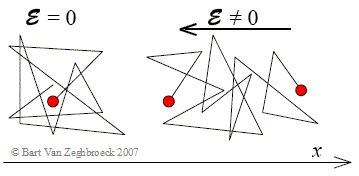
An electron in an electric field experiences a force.
-
This force causes the electron (which has mass) to accelerate.
-
Why does this not therefore cause an increasing current in a material?
Think about this question, then <click to reveal>
The electrons are scattered by the solid — always accelerating but constantly getting knocked off track.
Notice in this video during the Plinko game (around 3:00), the camera pans downward at an approximately constant rate: YouTube: The Price is Right former biggest Plinko win primetime.
This results in an average velocity which is constant even though an individual electron is always accelerating.[1]
The average electron velocity is proportional to the applied E-field.
The constant of proportionality is called mobility (μn for electrons and μp for holes) and must have units of \(\mathrm{\frac{cm^2}{V\cdot s}}\).
For silicon, these values are around:
-
\(\mu_n = 1350 \; \mathrm{\frac{cm^2}{V\cdot s}}\)
-
\(\mu_p = \phantom{1} 480 \; \mathrm{\frac{cm^2}{V\cdot s}}\)
Recall that the electric potential difference that we commonly name by its units of volts is only and truly the path integral of the electric field. Fortunately, the E-field is a conservative field, so the result of the integration only depends on the end points:
- For holes
-
\(\vec{v}_h = \mu_p \vec{E}\), movement in the same direction as the \(\vec{E}\) field vector.
- For electrons
-
\(\vec{v}_e = -\mu_n \vec{E}\), movement in the opposite direction as the \(\vec{E}\) field vector.
1.2. Current flow in a bar
Imagine a bar of silicon
Let’s begin by considering the current that flows due to electrons.
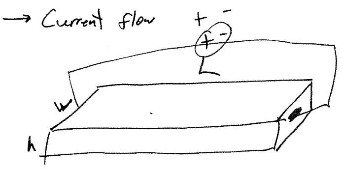

| Notice the double negative! Each negative has a different origin even though the net result is a positive sign. |
We know the electron (average) velocity, the density of (free) electrons, and the geometry of the bar. Let’s normalize this into a current flux by dividing by the cross-sectional area W·h.
| Jn has units of \(\mathrm{A / cm^2}\) which is the units of a flow per unit area or flux. In an unfortunate naming convention, everyone else calls this term electron current density. |
By the same reasoning, we can find the hole current density

The total current density is then
Finding the current that you would measure with an ammeter from this expression merely requires multiplying by the cross-section area of the bar.
But… look back at Figure 1, “Voltage source across a conductive bar” and see that we are applying a voltage across the ends of the bar (using an ideal voltage source) — what is \(\vec{E}\)?
An easy-ish way to remember what to do is to recall the units of the electric field: volts per meter. We get our voltage back by multiplyiing by meters, or the Length of the bar.
1.3. Mobility changes with doping :(
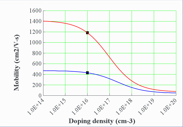
What causes this second-order effect? <think first, then click to reveal>
-
More doping means a less uniform crystal and more opportunities for scattering.
-
But (free) charge density increases faster than mobility decreases, so conductivity still increases.
1.4. Velocity saturation
It hopefully makes sense that the charge velocity can’t increase so much as to exceed the speed of light, so this is the obvious speed limit. (Light speed is about \(3\times 10^{10}\;\mathrm{cm/s}\))
The velocity (therefore current) approaches a lower limit and no longer varies linearly at large E-field strengths (voltage). In a circuit context, this means that the device changes from behaving like a resistor to more like a constant current source.[2] Velocity saturation is very common in modern integrated circuits.
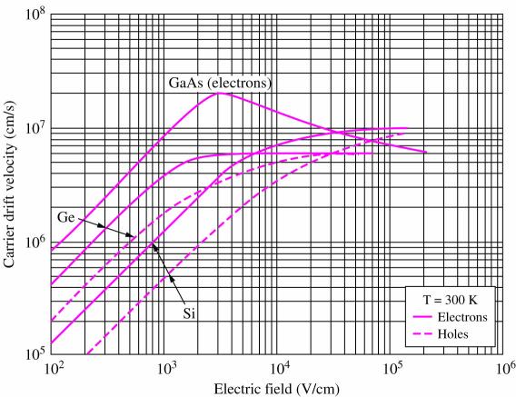
A \(130\,\mathrm{nm}\) chip process uses a \(1.2\,\mathrm{V}\) supply voltage, giving internal E-fields of
>>> print('%2.2g V/cm' % (1.2 / 130e-9 / 100) )

 9.2e+04 V/cm
which is well within the velocity saturation regime according to Drift velocity versus E-field. From Jaeger, Microelectronic Circuit Design.