1. Small-signal frequency response
The following document works through to the transfer function for a generic emitter-follower / common-collector amplifier. Its transfer function will be some polynomial in s of up to 3rd order since there are three reactive components in the circuit.
Consider this single-pole transfer function as an example for using Matlab to plot its frequency response.
%% Set independent frequency vector
% needs to cover the "special" frequency of 12

%            /-- start at w=0
%            |   /-- end at 1200 rad/s
%            |   |      /-- this many items
w = linspace(0, 1200, 1000);


%% Compute the complex-valued transfer function
% The transfer function example
%   Mind the difference between "/" and "./" !
%   If in doubt, always use "./" and ".*" and " .' "
A = 35 ./ (1 + 1j*w / 12);


%% Plot to see the *magnitude*
plot(w, abs(A))
labels('V/V')


%% Log-space the x-axis (frequency) only
semilogx(w, abs(A))
labels('V/V')

%% Log-space both axes to look even more familiar
loglog(w, abs(A))
labels('V/V')


%% Use decibels for the vertical axis
Amag_dB = 20*log10(abs(A));

% y-axis is *already* log-spaced, so only log-space the x-axis
semilogx(w, Amag_dB)
labels('dB')

fprintf("\nMax gain %.1f V/V\n", max(abs(A)))
fprintf("Max gain %.1f dB\n", max(Amag_dB))


%% Helper functions

% Label the plot and add grid
function labels(y_units)
    grid('on')
    xlabel("Frequency \omega")
    ylabel(["Magnitude |A| ", y_units])
    title("Transfer function")
end
2. Design trade-offs and Pareto curves
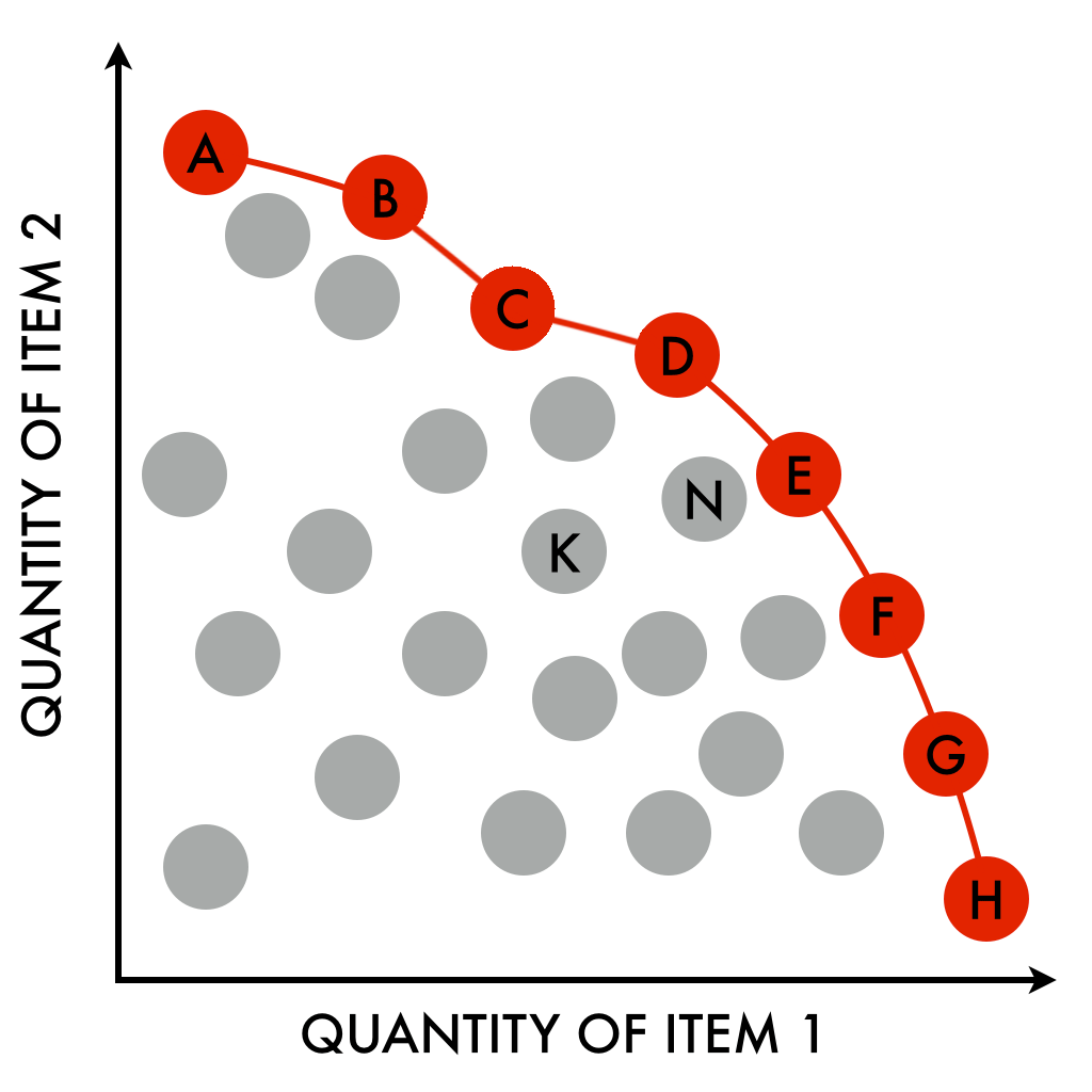
Economists and engineers have lots in common in how they view the relationship between decision variables.
-
efficiency (lots of types!) / inefficient
-
possible / unattainable
-
marginal rates (point slopes on a curve)
⇒ All solutions along a Pareto front(ier) are “the best”. Engineering decisions should choose one of these options.
⇒ Choosing an option that is NOT on the front means that you are “leaving something on the table”: there is an objectively better option!

3. Build vs. Buy op amps
Building your own operational amplifier is fun and interesting, but the days of making your own custom opamp to obtain specific performance in a design are increasingly rare.
-
Understand the specifications that are most important for your specific design’s needs.
-
Search for models that meet those specs.
-
Select the "best" from that group. (What is best???)
The linked and printed table shows a good selection of amplifiers that are either common or quite good in their respective optimizations. New ones are introducted all the time, and old ones go out of production!